EE274 (Fall 23): Homework-2

• Focus area: Lossless Compression
• Due Date: Nov 1, midnight (11:59 PM)
• Weightage: 15%
• Total Points: 110

Q1: Camping Trip (20 points)

During one of the camping trips, Pulkit was given $n$ rope segments of lengths $l_1,l_2,\dots ,l_n$ by Kedar, and was asked to join all the ropes into a single long segment of length ${\sum }_{i=1}^n{l}_i$. Pulkit can only join two ropes at a time and the "effort" in joining ropes $i,j$ using a knot is $l_i+l_j$. Pulkit is lazy and would like to minimize his "effort" to join all the segments together.

1. [5 points] Do you see any parallels between the problem and one of the prefix-free codes you have learnt about? Please justify your answer.

   Solution

   Yes, the problem is connected to Huffman Codes. The cost of joining a rope into the final segment is proportional to number of times it is used in the knotting process. We will need to pay a larger penalty for a rope if it is used for creating a knot earlier, than later. We can visualize the process of creating the final long segment as a prefix-free tree construction where nodes represent the cost of joining the ropes and depth of the node indicates how many times the particular rope corresponding to this node was used for creating the final segment. Mathematically, the problem is same as

   $$\underset{\text{prefix-free code}}{\min }\sum _{i=1}^n{l}_i\cdot d_i$$

   where $l_i$ is the length of the rope and $d_i$ is the number of times the rope is knotted.

   We have seen this optimization problem before in class when we were constructing Huffman tree!

2. [5 points] Let $E_{opt}$ be the optimal (minimal) value for the effort required to join all the segments. Without solving the problem, can Pulkit get an estimate of what the $E_{opt}$ would be? Leaving your answer in terms of inequalities is fine.

   Solution

   To map the problem precisely to Huffman Tree construction as seen in class, we need to ensure that we are optimizing over probability distribution over ropes. This can be trivially done by normalizing the rope lengths. Let $p_i=\frac{l_i}{{\sum }_{i=1}^n{l}_i}$ be the probability corresponding to Huffman tree for rope $i$. Then, the problem can be mapped to the following optimization problem:

   $$\underset{\text{prefix-free code}}{\min }\left(\sum _{i=1}^n{p}_i\cdot d_i\right)\times \left(\sum _{i=1}^n{l}_i\right)$$

   Note that ${\sum }_{i=1}^n{p}_i=l_i$ is constant given rope-lengths. We can now use the fact that the optimal value of the above optimization problem is equal to the entropy of the probability distribution over ropes $H(P)$ scaled by the sum of rope-lengths. Therefore,

   $$\left(\sum _{i=1}^n{l}_i\right)\cdot H(P)\le E_{opt}\le \left(\sum _{i=1}^n{l}_i\right)\cdot \left(H(P)+1\right)$$

   where $H(P)={\sum }_i{p}_i{\log }_2\frac{1}{p_i}$ is the entropy of the probability distribution over ropes as defined above.

3. [10 points] Implement the function compute_minimum_effort() in the file hw2_p1.py.
   HINT: You may use one of the prefix-free code implementations in the SCL Library

   Solution

   def compute_minimal_effort(rope_lengths_arr: List[float]) -> float:
   """
   lengths_arr -> list of rope lengths (positive floating points)
   output -> the value of the minimum effort in joining all the ropes together 
   """
   effort = None
   ###########################################################
   # Q5.3: Add code here to compute the minimal effort
   ###########################################################
   # raise NotImplementedError
   
   from compressors.huffman_coder import HuffmanTree
   from core.prob_dist import ProbabilityDist
   
   # create a prob_dist out of the rope_lengths_arr
   rope_lengths_dict = {f"rope_id_{ind}": val for ind, val in enumerate(rope_lengths_arr)}
   prob_dist = ProbabilityDist.normalize_prob_dict(rope_lengths_dict)
   encoding_table = HuffmanTree(prob_dist).get_encoding_table()
   
   # compute minimal effort as the average codelength of huffman code
   effort = 0
   for rope_id in encoding_table:
       effort += len(encoding_table[rope_id]) * rope_lengths_dict[rope_id]
   
   ###########################################################
   return effort  
   

Q2: Generating random non-uniform data (25 points)

Consider the problem of sampling a non-uniform discrete distribution, when you given samples from a uniform distribution.

Let's assume that we are given a single sample of random variable U, uniformly distributed in the unit interval [0,1) (e.g. U = numpy.random.rand()). The goal is to generate samples from a non-uniform discrete distribution $P$. We will assume that $P$ is a rational distribution. i.e. for any symbol $s$, $P(s)=n_s/M$, where $n_s,M$ are integers.

1. [5 points] Given a non-uniform rational distribution, we can sample a single random value $X_1\sim P$ from U by finding the cumulative distribution bin in which the sample U falls since the cumulative distribution also lies between [0,1). For example, if $P$ is the distribution such as P = {A: 2/7, B: 4/7, C: 1/7}, then we output the symbols A,B,C based on the intervals in which they lie as follows:

   if U in [0.0, 2/7) -> output A
   if U in [2/7, 6/7) -> output B
   if U in [6/7, 1.0) -> output C
   

   Generalize the above algorithm to any given rational distribution, and describe it in a few lines. For a distribution of alphabet size $k$ (e.g. $k=3$ in the example above), what is the time/memory complexity of your algorithm wrt $k$?

   Solution

   We can use the cumulative distribution function to find the bin in which the sample U falls and output the sample corresponding to that bin. The cumulative distribution function is defined as: $F(x)={\sum }_{i=1}^{x}P(i)$. We can find the bin in which the sample U falls by finding the smallest $x$ such that $F(x)>U$ and then output symbol x. We can use binary search for finding the bin. The time complexity of this algorithm is $O(log(k))$, where $k$ is the size of the alphabet. The memory complexity is $O(k)$, since we need to store the cumulative distribution function.

2. [5 points] Complete the function generate_samples_vanilla in hw2_p2.py which takes in a non-uniform rational distribution P and returns data_size number of samples from it. You can assume that the distribution is given as a dictionary, where the keys are the symbols and the values are the frequency of occurrence in the data. For example, the distribution P = {A: 2/7, B: 4/7, C: 1/7} can be represented as P = Frequencies({'A': 2, 'B': 4, 'C': 1}). Ensure that your code passes the test_vanilla_generator test in hw2_p2.py. Feel free to add more test cases.

   Solution

   def generate_samples_vanilla(freqs: Frequencies, data_size):
       """
       Generate data samples with the given frequencies from uniform distribution [0, 1) using the basic approach
       :param freqs: frequencies of symbols (see Frequencies class)
       :param data_size: number of samples to generate
       :return: DataBlock object with generated samples
       """
       prob_dist = freqs.get_prob_dist()
   
       # some lists which might be useful
       symbol_list = list(prob_dist.cumulative_prob_dict.keys())
       cumul_list = list(prob_dist.cumulative_prob_dict.values())
       cumul_list.append(1.0)
   
       generated_samples_list = []  # <- holds generated samples
       for _ in range(data_size):
           # sample a uniform random variable in [0, 1)
           u = np.random.rand()
   
           ###############################################
           # ADD DETAILS HERE
           ###############################################
   
           # NOTE: side="right" corresponds to search of type a[i-1] <= t < a[i]
           bin = np.searchsorted(cumul_list, u, side="right") - 1
           s = symbol_list[bin]
           generated_samples_list.append(s)
           ###############################################
   
       return DataBlock(generated_samples_list)
   

3. [5 points] Given a single sample of a uniform random variable U, how can you extend your algorithm in part 2.1 above to sample $n=2$ i.i.d random values $X_1,X_2\sim P$? Provide a concrete algorithm for P= {A: 2/7, B: 4/7, C: 1/7}. Generalize your method to an arbitrary number of samples $n$ and describe it in a few sentences.

   Solution

   We can sample $n$ i.i.d random values $X_1,X_2,\dots ,X_n\sim P$ by first calculating the cumulative distribution corresponding to all possible symbols of block length n and then following the procedure as described above. Note this method scales very poorly with n since the size of the alphabet increases exponentially with n.

4. [5 points] Pulkit suggested that we can slightly modify Arithmetic Entropy Coder (AEC) we learnt in the class to sample a potentially infinite number of i.i.d samples $X_1,X_2,\dots ,X_n\sim P$ given any rational distribution $P$ from a single uniform random variable sample U! You can look at Pulkit's implementation generate_samples_aec in hw2_p2.py to get an idea of how to exploit AEC. Can you justify the correctness of Pulkit's method in a few lines?

   Note: Even though we say that we can sample potentially infinite number of samples, in practice we are limited by the precision of floats.

   Solution

   Pulkit's solution first samples a random number U in $[0,1)$ and then truncates it to 32 bits. Then it artificially considers the truncated sample as the output of an arithmetic encoder coming from data with same probability as distribution we want to sample from. Finally, it outputs a random bit sequence based on the output of arithmetic decoding on this encoded bitstream. The scheme works because we know that the probability of the uniform random variable lying in an interval in $[0,1)$ is proportional to the interval length and an arithmetic encoder-decoder pair works by dividing the number line between $[0,1)$ in interval lengths proportional to the probability of corresponding n-block symbols. Therefore, we can recover an arbitrary n bit symbol (upto precision of floats) with correct probabilities as given distribution by simply using arithmetic encoding followed by arithmetic decoding.

5. [5 points] Now let's say that you have to sample data $X_0,X_1,\dots ,X_n$ from a Markov distribution $Q$. Recall for a Markov Chain, $Q(X_0,X_1,\dots ,X_n)=Q(X_0)Q(X_1|X_0)\dots Q(X_n|X_{n-1})$. Can you use your technique from Q2.3 or the technique suggested by Pulkit in Q2.4 to sample any number of samples $n$ with Markov distribution $Q$ from a single uniform random variable sample U in [0,1)? Describe the algorithm in a few lines.

   Solution

   We can use either of the techniques in Q2.3 or Q2.4 to sample from a markov chain by simply modifying the probability distribution of n-block symbols to be the markov chain distribution. For example, we can use technique in Q2.3 by calculating the cumulative distribution corresponding to all possible symbols of block length n using the described markov chain probability decomposition and then following the procedure as described in Q2.3. We can use technique in Q2.4 by considering the truncated sample as the output of an arithmetic encoder coming from data with same probability as markov chain distribution we want to sample from. In this case, we'll use the conditional distribution at each arithmetic decoding step as we did in lecture 9.

Q3: Conditional Entropy (20 points)

In this problem we will get familiar with conditional entropy and its properties.

We learnt a few properties of conditional entropy in class:

• $H(X)\ge H(X|Y)$
• $H(X,Y)=H(Y)+H(X|Y)$

We will use these properties to show some other useful properties about conditional entropy and solve some fun problems!

1. [5 points] Let $f(X)=Z$ be an arbitrary function which maps $X\in \mathcal{X}$ to a discrete set $Z\in \mathcal{Z}$. Then show that: $H(f(X)|X)=0$. Can you intuitively explain why this is the case?

   Solution

   Given a value of $X=x$, $f(X)$ has a deterministic value $f(x)$. Therefore $H(f(X)|X=x)=0$ and

   $H(f(X)|X)={\sum }_{x}p(x,f(x))H(f(X)|X=x)={\sum }_{x}0$

2. [5 points] Show that $H(f(X))\le H(X)$, i.e. processing the data in any form is just going to reduce the entropy. Also, show that the equality holds if the function $f$ is invertible, i.e. if there exists a function $g$ such that $g(f(X))=X$. Can you intuitively explain why this is the case?

   Solution

   Let's use the chain rule of entropy in two different ways:

   $$\begin{array}{rl}H(X,f(X))& =H(X)+H(f(X)|X)=H(X)\\ H(X,f(X))& =H(f(X))+H(X|f(X))\ge H(f(X))\end{array}$$

   since $H(f(X)|X)=0$ and $H(X|f(X))\ge 0$. Therefore, $H(X)\ge H(f(X))$.

   The equality holds when $H(X|f(X))=0$. This holds when $X$ is a deterministic function of $f(X)$ implying that $f(X)$ is invertible. Intuitively, if there is a one-to-one mapping between $X$ and $f(X)$, then the entropy of $X$ is the same as the entropy of $f(X)$ as all we are doing is changing the alphabets but not the probability distribution across those alphabets!

3. [4 points] In the HW1 of the 2023 edition of EE274, Pulkit and Shubham had an assignment to compress the Sherlock novel (lets call it $x_{orig}$). Pulkit computed the empirical 0th order distribution of the letters and used those with Arithmetic coding to compress $x_{orig}$, and received average codelength $L_1$. While working on the assignment, Shubham accidentally replaced all letters with lowercase (i.e A -> a, B -> b etc.). Lets call this modified text $x_{lowercase}$. Shubham compressed $x_{lowercase}$ with the same algorithm as Pulkit, and got average codelength $L_2$. Do you expect $L_1\ge L_2$, or $L_2\ge L_1$. Justify based on properties of Arithmetic coding and Q3.2.

   Solution

   We know that $H(X)\ge H(f(X))$. Since Shubham replaced all capital letters with lowercase, the operation can only reduce the entropy, i.e. $H(x_{orig})\ge H(x_{lowercase})$. We also know that arithmetic coder achieves entropy of any given probability distribution, and hence, $L_1\ge L_2$.

4. [6 points] We say that random variables $X_1,X_2,\dots ,X_n$ are pairwise independent, if any pair of random variables $(X_i,X_j),i\ne j$ are independent. Let $X_1,X_2,X_3$ be three pairwise independent random variables, identically distributed as $Ber(\frac{1}{2})$. Then show that:

   1. [3 points] $H(X_1,X_2,X_3)\le 3$. When is equality achieved?
   2. [3 points] $H(X_1,X_2,X_3)\ge 2$. When is equality achieved?

   Solution

   Using chain rule of entropy and the fact that $X_i$ are pairwise independent, we have:
   $$\begin{array}{rl}H(X_1,X_2,X_3)& =H(X_1)+H(X_2|X_1)+H(X_3|X_1,X_2)\\ & =H(X_1)+H(X_2)+H(X_3|X_1,X_2)\\ & =1+1+H(X_3|X_1,X_2)\\ & =2+H(X_3|X_1,X_2)\end{array}$$

   where $H(X_2|X_1)=H(X_1)$ since $X_2$ and $X_1$ are independent. But note that, $H(X_3|X_1,X_2)$ need not be always $0$ as our random variables are pairwise independent but need not be mutually independent! Third line follows from the fact that $X_i$ are $Bern(0.5)$ and hence $H(X_i)=1$.

   a. To show this note that: $H(X_3|X_1,X_2)\le H(X_3)=1$, since conditioning reduces entropy. This equality is achieved when $X_3$ is independent of $X_1$ and $X_2$, i.e. random variables are mutually independent.
   b. To show this note that: $H(X_3|X_1,X_2)\ge 0$, since entropy is always positive. From Q1.1 this equality is achieved when $X_3$ is a function of $X_1,X_2$. Since the marginal distribution of $X_3$ is $Bern(0.5)$, you can show that only function which satisfies this property is $X_3=X_1\oplus X_2$.

5. [NOT GRADED, THINK FOR FUN!] Let $Z_1,Z_2,\dots ,Z_k$ be i.i.d $Ber(\frac{1}{2})$ random variables. Then show that using the $Z_i^{\prime }s$, you can generate $n=2^k-1$ pairwise independent random variables, identically distributed as $Ber(\frac{1}{2})$.

   Solution

   Consider all possible xor combinations of $Z_i$, i.e. $Z_1,Z_2,\dots ,Z_k,Z_1\oplus Z_2,Z_1\oplus Z_3,Z_2\oplus Z_3,\dots ,Z_1\oplus Z_2\oplus Z_3\oplus \dots \oplus Z_k$. We can see that each of these random variables are pairwise independent since $Z_i$ are i.i.d. and $Bern(0.5)$. Hence, we can generate $n=2^k-1$ pairwise independent random variables, identically distributed as $Bern(0.5)$.

Q4: Bits-Back coding and rANS (45 points)

In class, we learnt about rANS. We started with the basic idea of encoding a uniform distribution on {0, ..., 9} (see Introduction section in notes) and then extended it to non-uniform distributions. In this problem we will look at a different way of thinking about rANS, which will help us understand the modern entropy coder.

Let's start by first generalizing our idea of encoding a uniform distribution on {0, ..., 9} to a uniform distribution on {0, ..., M-1}, where M can be thought of as number of symbols in the alphabet. The encoding works as following:

def encode_symbol(state, s, M):
    state = (state * M + s) 
    return state

The encoder maintains a single state, which we increase when we encode a symbol. Finally, we save the state by simply writing it out in the binary form. This function is implemented in hw2_p4.py as UniformDistEncoder.

1. [2 points] Write a decode_symbol pseudocode which takes in the encoded state state and M and returns the symbol s and the updated state state. Show that your decoder along with above encoding is lossless, i.e. we can recover the original symbol s from the encoded state state and M.

   Solution

   def decode_symbol(state, M):
       s = state % M
       state = state // M
       return s, state
   

   Since the state input into the decoder is state = state_prev * M + s with 0 <= s < M, then (state_prev * M + s) % M = s. Therefore, we can recover the original symbol s from the encoded state state and M. And the previous state is then just (state_prev * M + s) // M.

2. [3 points] Show that given data in {0, ..., M-1}, the encoder/decoder pair can be used to achieve lossless compression with ~ log2(M) bits/symbol as we encode large number of symbols.

   Solution

   Just like in the case where M=10 we discuss in the course notes, the size of the state increases by a factor of M for every symbol we encode, plus an addition of s. After some time, this s term will be small relative to the state, which is several powers of M larger, so in the limit of a large number so symbols, we can ignore the s term. and the number of bits required to encode the state is log2(M) times the number of symbols encoded.

3. [5 points] Now, implement your decoder in hw2_p4.py as UniformDistDecoder. Specifically, you just need to implement decode_op function. Ensure that your code passes the test_uniform_coder test in hw2_p4.py. Feel free to add more test cases.

   Solution

   def decode_op(state, num_symbols):
   '''
   :param state: state
   :param num_symbols: parameter M in HW write-up
   :return: s, state_prev: symbol and previous state
   '''
   s = state_prev = None
   ####################################################
   # ADD CODE HERE
   # raise NotImplementedError
   ####################################################
   s = state % num_symbols
   state_prev = state // num_symbols
   
   return s, state_prev
   

Now, we want to implement a compressor which works well for non-uniform data. We will use the base encode/decode functions from UniformDistEncoder, UniformDistDecoder and approach this problem from a new perspective. In class, we learned $H(X,Z)=H(X)+H(Z|X)$ for any two random-variables $X$ and $Z$. We will use this property to encode the data $X$. Note that this identity implies $$H(X)=H(X,Z)-H(Z|X)$$

Interpreting this intuitively, it should be possible to encode data X in following two steps:

a. Encode X,Z together using a joint distribution P(X,Z). Assuming an ideal compressor, this will require H(X,Z) bits.

b. Decode H(Z|X) from the encoded state using distribution P(Z|X). Again, assuming an ideal compressor, this lets us recover H(Z|X) bits.

Step b gives you an intuition for the question name -- bits-back! Here Z is an additional random variable typically latent variable (latent means hidden). Be careful while reading this step, as it is not a compressor for X but a decompressor for Z|X! This compressor assumes knowledge of X and decodes Z from the encoded state. More concretely, we will have an encoder-decoder pair which will work as follows:

def encode_symbol(state, X):
    state, Z = decode_zgx(state, X) # decode Z|X from state; knows X. returns Z and updated state.
    state = encode_xz(state, (X, Z)) # use this Z, and known X, to encode X,Z together. returns updated state.
    
    return state


def decode_symbol(state):
    state, (X, Z) = decode_xz(state) # decode X,Z from state. returns X,Z and updated state.
    state = encode_zgx(state, Z, X) # encode Z|X by updating state; knows X. returns updated state.
    
    return state, X

Note that how the encode step now involves both a decoding and an encoding step from another compressor! This is one of the key idea behind bits-back coding. We will now implement the above encoder/decoder pair for non-uniform data.

To see the idea, let's work out a simple case together. As usual let's assume that the non-uniform input is parametrized by frequencies freq_list[s] for s in {1,..,num_symbols} and M = sum(freq_list). For instance, if we have 3 symbols A,B,C with probabilities probs = [2/7, 4/7, 1/7], then we can think of frequencies as freq_list = [2,4,1] and M = 7. We can also create cumulative frequency dict as we saw in class, i.e. cumul = {A: 0, B: 2, C: 6}.

We will assume Z to be a uniform random variable in {0, ..., M-1}. Then, we can think of X as a function of Z as follows:

def X(Z):
    for s in symbols:
        if cumul(s) <= Z < cumul(s) + freq_list[s]:
            return s

i.e. X is the symbol s such that Z lies in the interval [cumul(s), cumul(s)+freq_list[s]). This is shown in the figure below for the example above.

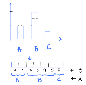
For example if Z = 4, then X = B as cumul(B) = 2 <= 4 < 6 = cumul(B) + freq_list[B].

4. [2 points] What are the values of $H(X),H(Z),H(X|Z)$ in the above example?

   Solution $$H(X)=-(\frac{2}{7}\log \frac{2}{7}+\frac{4}{7}\log \frac{4}{7}+\frac{1}{7}\log \frac{1}{7})\approx 1.378783$$ $$H(Z)=-\log \frac{1}{M}=\log M\approx 2.81$$ $$H(X|Z)=\sum _{z=0}^{M-1}p(z)H(X|Z=z)=-\sum _{z=0}^{M-1}p(z)\sum _{x\in X}p(x|z)\log p(x|z)$$

   Notice that $p(x|z)=1$ if $x=X(z)$ and $0$ otherwise. If $p(x|z)=0$, then the term $p(x|z)\log p(x|z)$ in the sum is also $0$, and if $p(x|z)=1$, then $\log p(x|z)=0$, and the term also disappears, since this is true for all terms in the sum, $H(X|Z)=0$. In general, for some variable, $Y$, $H(f(Y)|Y)=0$ for any function $f$. This is because f(Y) is completely determined by $Y$, so given $Y$, there is no uncertainty in $f(Y)$ and the entropy is 0.

5. [3 points] What is the distribution and entropy of $Z$ given $X$, i.e. $P(Z|X)$ and $H(Z|X=x)$ in the above example? Note that $H(Z|X=x)$ is a function of x and hence you need to report it for each symbol x in the alphabet A,B,C.

   Solution Notice that given a value of $X=x$, $Z$ is uniformly distributed over the range of $x$. So,

   $$\begin{array}{rl}P(Z=z\mid X=A)& =\{\begin{array}{ll}\frac{1}{2}& z\in [0,1]\\ 0& \text{ else }\end{array}\\ P(Z=z\mid X=B)& =\{\begin{array}{ll}\frac{1}{4}& z\in [2,3,4,5]\\ 0& \text{ else }\end{array}\\ P(Z=z\mid X=C)& =\{\begin{array}{ll}1& z\in [6]\\ 0& \text{ else }\end{array}\end{array}$$

   This means that the conditional entropy $H(Z|X)$ for X \in [A,B,C] is just that of a uniform distribution over 2, 4, and 1 possibilities, respectively. So,

   $$\begin{array}{rl}H(Z|X=A)& =-{\log }_2\frac{1}{2}={\log }_{2}2=1\\ H(Z|X=B)& =-{\log }_2\frac{1}{4}={\log }_{2}4=2\\ H(Z|X=C)& =-{\log }_{2}1=0\end{array}$$

   (if you are curious) The full calculation of $H(Z|X)$ is shown below:

   $$\begin{array}{rl}H(Z|X)& =\sum _{x\in \left[A,B,C\right]}p(x)H(Z|X=x)=-\sum _{x\in \left[A,B,C\right]}p(x)\sum _{z=0}^{M-1}p(z|x)\log p(z|x)\\ & =p(x=A)H(Z|X=A)+p(x=B)H(Z|X=B)+p(x=C)H(Z|X=C)\\ & =-(\frac{2}{7}({\log }_2\frac{1}{2})+\frac{4}{7}({\log }_2\frac{1}{4})+\frac{1}{7}({\log }_{2}1))\\ & =\frac{2}{7}+\frac{4}{7}\ast 2=\frac{10}{7}\approx 1.428571\end{array}$$

Now, let's implement the encoder/decoder pair for the above example. We will use the following notation:

• state is the encoded state
• s is the symbol to be encoded (X)
• freq_list is the list of frequencies of the symbols
• We want to code the above scheme utilizing the joint compressors over X, Z (where Z is the latent variable). Z is uniformly distributed in {0, ..., M-1}.
  • combined_symbol is the joint random variable Y = (X, Z). In our example, we only need to encode Z as X is a deterministic function of Z, i.e. combined_symbol = Z and will be in {0, ..., M-1}. For above example, say we want to encode Y = (B, 4), then we only need to encode Z = 4 as X=B is implied.
  • fake_locator_symbol is the value of Z|X=x relative to cumul(x). This is a function of X=x. For above example of X = B, Z|X=B can be {2, 3, 4, 5} and hence fake_locator_symbol can be {0, 1, 2, 3} respectively as cumul(B) = 2.
  • Therefore, combined_symbol and fake_locator_symbol allows us to have encoder/decoder pair for both (X,Z) and Z|X. Continuing our example, if we were to encode Y = (X=B, Z=4), we will encode it as combined_symbol = 4 and fake_locator_symbol = 2. Conversely, if we were to decode combined_symbol = 4, we will decode it as Y = (Z=4, X=B) and infer that fake_locator_symbol=2.

6. [5 points] We have implemented the encode_symbol function for NonUniformDistEncoder. Looking at the pseudocode above and the example, explain briefly how it works. Specifically, explain how encode_symbol achieves the relevant decode_zgx and encode_xz functions given in pseudocode in the context of example above.

   Solution encode_symbol is shown below:

def encode_symbol(self, x, state):
    '''
    :param x: symbol
    :param state: current state
    :return: state: updated state
    '''
    # decode a "fake" uniform sample between [0, freq[x]]
    fake_locator_symbol, state = decode_op(state, self.freq.freq_dict[x])
    # print(s, fake_locator_symbol, state)
    # create a new symbol
    combined_symbol = self.freq.cumulative_freq_dict[x] + fake_locator_symbol

    # encode the new symbol
    state = encode_op(state, combined_symbol, self.freq.total_freq)
    # print(state)
    # print("*" * 5)
    return state

By using decode_op from our UniformDistDecoder, we can decode a "fake" uniform sample between [0, freq[x]]. We then add this to the cumulative frequency of x to get the value of Z, which we encode as combined_symbol (see the first bullet point above). We can now encode the state, encode_op with the value of Z being used for s. decode_zgx is accomplished by the first two lines where we pass the function the state and the value of X and decode Z (which is stored as combined_symbol), and update the state. Then, encode_xz is accomplished by the last line by feeding encode_op the state, Z and X.

7. [10 points] Now implement the decode_symbol function for NonUniformDistEncoder. You can use the encode_op and the decode_op from uniform distribution code. Ensure that your code passes the test_non_uniform_coder test in hw2_p4.py. Feel free to add more test cases.

   Solution

       def decode_symbol(self, state):
           '''
           :param state: current state
           :return: (s, state): symbol and updated state
           '''
           #################################################
           # ADD CODE HERE
           # a few relevant helper functions are implemented:
           # self.find_bin, self.freq.total_freq, self.freq.cumulative_freq_dict, self.freq.freq_dict, self.freq.alphabet
   
           # Step 1: decode (s, z) using joint distribution; (i) decode combined symbol, (ii) find s
           # Step 2: encode z given s; (i) find fake locator symbol, (ii) encode back the fake locator symbol
   
           # You should be able to use encode_op, decode_op to encode/decode the uniformly distributed symbols
   
           # decode combined symbol
           combined_symbol, state = decode_op(state, self.freq.total_freq)
           cum_prob_list = list(self.freq.cumulative_freq_dict.values())
           decoded_ind = self.find_bin(cum_prob_list, combined_symbol)
           s = self.freq.alphabet[decoded_ind]
   
           # find fake locator symbol
           fake_locator_symbol = combined_symbol - self.freq.cumulative_freq_dict[s]
   
           # encode back the fake locator symbol
           state = encode_op(state, fake_locator_symbol, self.freq.freq_dict[s])
   
           #################################################
           return s, state
   

8. [5 points] Show that for a symbol s with frequency freq[s], the encoder uses ~ log2(M/freq[s]) bits and is hence optimal.

   Solution

   For a symbol, s, the function encode_symbol(s,state) first divides the input state by freq[s] in the line fake_locator_symbol, state = decode_op(state, self.freq.freq_dict[s]). Then, the state is multiplied by M in the line state = encode_op(state, combined_symbol, self.freq.total_freq). So, in each step of the encoding, we scale by M/freq[s], so in the limit of a large number of symbols, we require log2[M/freq[s]] bits to encode a state.

Great, we have now implemented a bits-back encoder/decoder pair for a non-uniform distribution. Let us now see how it is equivalent to rANS we studied in class. As a reminder, the rANS base encoding step looks like

def rans_base_encode_step(x,s):
   x_next = (x//freq[s])*M + cumul[s] + x%freq[s]
   return x_next

9. [5 points] Justify that encode_symbol in NonUniformDistEncoder performs the same operation as above.

   Solution Let's walk through the transformation of the state in encode_symbol step-by-step. First off, fake_locator_symbol, state = decode_op(state, self.freq.freq_dict[s]) proforms the transformation state -> state // freq[s] and gives fake_locator_symbol = state%freq[s]. Then the line state = encode_op(state, combined_symbol, self.freq.total_freq) performs the transformation state // freq[s] -> (state // freq[s])*M + combined_symbol, but combined_symbol = self.freq.cumulative_freq_dict[s] + fake_locator_symbol = cumul[s] + state%freq[s], so overall we have state -> (state // freq[s])*M + cumul[s] + state%freq[s]. This is exactly the same as the rANS base encoding step, so encode_symbol performs the same operation as the rANS base encoding step.

Similarly, as a reminder, the rANS base decoding step looks like

def rans_base_decode_step(x):
   # Step I: find block_id, slot
   block_id = x//M
   slot = x%M
   
   # Step II: Find symbol s
   s = find_bin(cumul_array, slot) 
   
   # Step III: retrieve x_prev
   x_prev = block_id*freq[s] + slot - cumul[s]

   return (s,x_prev)

10. [5 points] Justify that decode_symbol in NonUniformDistEncoder performs the same operation as above.

    Solution combined_symbol = state % M and state = state//M, so combined_symbol = slot and state = block_id. Then decoded_ind = self.find_bin(cum_prob_list, combined_symbol) and s = self.freq.alphabet[decoded_ind] implement s = find_bin(cumul_array, slot). Finally, state = encode_op(state, fake_locator_symbol, self.freq.freq_dict[s]) performs the transformation state -> state*freq[s] + fake_locator_symbol, but fake_locator_symbol = combined_symbol - self.freq.cumulative_freq_dict[s], so we have state -> (state//M)*freq[s] + state % M - cumul[s] for the whole function, which is the same as the rANS base decoding step.

Therefore, bits-back coding is equivalent to rANS! Thinking again in terms of $H(X)=H(X,Z)-H(Z|X)$, it allows us to interpret rANS in terms of latent variables $Z$ in a more intuitive way. This question was highly motivated by the IT-Forum talk by James Townsend in 2022. Check out the YouTube video if you are interested to learn more!